Assignment #1
Due on Github 23:59 Wednesday 16 August
Goals
- introduce neural networks in terms of more basic ideas: linear regression and linear-threshold classification.
- Code up the simplest actual neural network, Rosenblatt’s Perceptron
Part 0: NumPy warmup
If you’re already familiar with NumPy, the numerical package we’ll use throughout this course, you can probably skip ahead to Part 1. Otherwise, fire up IDLE3 or your favorite Python3 interpreter, and do this:
>>> import numpy as np
Now we can just use the abbreviation np whenever we want to use something from NumPy. For example, we can create an empty array like this:
>>> x = np.array([])
To append a value v to the array:
>>> x = np.append(x, v)
The power of NumPy is its ability to perform a single operation on an entire array at once. For example:
>>> sum(x*x)
will return the sum of all the squared values in array x. NumPy also adds the power of types (as in Java or C++) to your computations. The following code shows how you can use types to switch back and forth between boolean (True/False) and numerical (1/0) arrays:
     >>> model    = np.array([5, 1, 2, 3, 4])
     >>> obtained = np.array([5, 6, 2, 3, 2])
     >>> model == obtained
     array([ True, False,  True,  True, False], dtype=bool)
     >>> sum((model == obtained).astype('int')) / len(model)
     0.59999999999999998
Here we see that our obtained values are in 60% agreement with the values from our model, with the extra digits due to the inevitable rounding error. Using this information and your existing knowledge of Python, you should be able to complete this assignment without too much difficulty.
Part 1
Consider the following table that describes a relationship between two input variables x1, x2 and an output variable y.
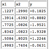
This is part of a larger data set that Prof. Michael Mozer created, which you can download in text format. Using Python and NumPy, write a program to read in the data file and find the individual least squares solutions to y=mx1+by=mx1+b and y=mx2+by=mx2+b. You can use the formulas from the lecture slides. Don’t modify the data file, because I will use the original version when testing your code.
Part 2
Now solve the full linear regression y=w1x1+w2x2+by=w1x1+w2x2+b using np.linalg.lstsq. Hint: The example they give can be modified slightly to do what we need. You should pass x1, x2 to np.vstack instead of just x. The output of np.linalg.lstsq(A, y)[0] will then be your w1, w2, b instead of the m, c in their example.
Part 3
Turn this data set from a regression problem into a classification problem by running each pair of points x1,x2x1,x2 through the regression equation. In other words, use w1x1+w2x2+b>0w1x1+w2x2+b>0 as a criterion for assigning each point x1,x2x1,x2 to one class or the other. You can then compare this classification to the values in the zz column of the dataset. Report your success rate as a percentage. If you do this right, your solution to Part 3 will require only a couple of lines of code added to the code you wrote for Part 2.
Part 4
In machine learning, we really want to train a model based on some data and then expect the model to do well on “out of sample” data. Try this with the code you wrote for Part 3: Train the model on the first {25, 50, 75} examples in the data set and test the model on the final {75, 50, 25} examples, reporting percentage correct for each size. As a baseline test, do a final report on percentage correct when w1=w2=b=0w1=w2=b=0.
Part 5
Write a module perceptron.py based on slides #3 and #4 of the lecture notes. Your module should of course start by importing NumPy:
import numpy as np
Your module should then define a class Perceptron. As usual when creating a Python class, you should first define an __init__ method and a __str__ method. The __init__ method should allow you to specify the number of inputs n and the number of outputs m, which will be instance variables for the class. Once you’ve got that part of __init__ written, you can write the __str__ method. This method should return a string with some useful info about the perceptron; for example, A perceptron with 5 inputs and 3 outputs.What other instance variables do we need to represent the state of our perceptron? Weights, of course! Here’s where we start using NumPy. Looking at the Perceptron Learning Algorithm in slide #6, you see that it initializes the weights as an (n+1) ×m matrix of small random numbers above and below 0. Looking over your NumPy warmup above, it should be pretty obvious how to do this: instead of multiplying by 2 and subtracting 1, figure out appropriate values to get the w values between some small interval, like [-.05,+.05]. You can debug your perceptron by printing out the weights at the end of your __init__, but make sure to get rid of that debugging output once you’ve got the init working. Or, you could have your __str__method return a a string representation of the weights, although this will become impractical for larger perceptrons.
Before we can train our perceptron to do anything interesting, we need a way of testing it in a given input. So add a method test. In a single line of code, this method should take an input vector (numpy array) I, append a 1 to it for the bias term (use np.append), perform the np.dot operation on it and the perceptron’s weights, compare the resulting vector with 0, and return the result.
Now that you’ve got your test method written, how should you test the test? As usual with software testing, it’s best to make sure it works as expected on a few simple, extreme cases. The simplest possible perceptron would have a single input and a single output (m = n = 1). This will give you just two weights. By examining the weights, you should be able to tell ahead of time what the test method will output on the two extreme values of the input: an input of 0 and an input of 1. Keep creating and testing this tiny perceptron until you get one that distinguishes an input of 0 from an input of 1. Once you’ve got that working, try a perceptron with two inputs instead of one. You can use np.zeros and np.ones to create an input vector of all 0s or 1s. Do the same validation as you did with the one-input perceptron, looking at the weights to make sure the output makes sense. Repeat with a perceptron of one input and two outputs, then finally two inputs and two outputs. If you can verify the results with these simple cases, there’s unlikely to be anything wrong with your test method.
Finally, it’s time to write the train method. This method should take two parameters: a NumPy matrix of input patterns (one pattern per row) and a NumPy matrix of target patterns (one per row), with the same number of rows as the input patterns. (Don’t worry about raising an exception if they have a different number of rows; you can that later if you like, after you’ve got the basics working.) You can use np.hstack for augmenting your input matrix with a final column of 1’s. Your train method should loop over the rows in the matrices, running the Perceptron Learning Algorithm from slide #6 of the lecture notes. For (Ij∗w)(Ij∗w) you can use np.dot as in the previous assignment. For ITj∗DjIjT∗Dj you can use np.outer. You can use 1000 iterations as a default, allowing your user to specify a different number by using a Python named argument for the third input to train. As with your test method, debug this method by using very simple functions (input/target sets). The Boolean functions AND and OR are the classic training examples for a perceptron, so try them (train/test one perceptron for OR, and another for AND). As with the previous assignment, I should be able to open your code in IDLE, hit F5, and see a nice clean printout showing me the trained perceptron’s behavior on each of the four inputs for these two Boolean functions.
It should be easy to get perfect results with these two simple functions (for reasons we will discuss in class). So you might want to add a third, optional parameter to your train method, niter=1000, for the number of iterations of the outer loop. Experiment with how small a number it takes for the weights to converge (stop giving a better result). For this part, I often got convergence / success in under five iterations.
Part 6
Our realistic data set consists of handprinted digits, originally provided by Yann Le Cun. Each digit is described by a 14×14 pixel array. Each pixel has a grey level with value ranging from 0 to 1. The data is split between two files, a training set that contains the examples used for training your neural network, and a test set that contains examples you’ll use to evaluate the trained network. Both training and test sets are organized the same way. Each file begins with 250 examples of the digit “0”, followed by 250 examples of the digit “1”, and so forth up to the digit “9”. There are thus 2500 examples in the training set and another 2500 examples in the test set.
Each digit begins with a label on a line by itself, e.g., “train4-17”, where the “4” indicates the target digit, and the “17” indicates the example number. The next 14 lines contain 14 real values specifying pixel intensities for pixels in the corresponding row. Finally, there is a line with 10 integer values indicating the target. The vector “1 0 0 0 0 0 0 0 0 0” indicates the target 0; the vector “0 0 0 0 0 0 0 0 0 1” indicates the target 9.
Write code to read in a file — either train or test — and build a data structure containing the input-output examples. Although the digit pixels lie on a 14×14 array, the input to your network will be a 196-element vector. The arrangement into rows is to help our eyes see the patterns. You might also write code to visualize individual examples.
Note: we will use the same data set in the next assignment when we implement back propagation, so the utility functions you write here will be reused. It’s worth writing some nice code to step through examples and visualize the patterns.
Part 7
Train a perceptron to discriminate 2 from not-2. That is, lump together all the examples of the digits {0, 1, 3, 4, 5, 6, 7, 8, 9}. You will have 250 examples of the digit 2 in your training file and 2250 examples of not-2. Assess performance on the test set and report false-positive and false-negative rates. The false-positive rate is the rate at which the classifier says “yes” when it should say “no” (i.e., the proportion of not-2’s which are classified as 2’s). The false-negative rate is rate at which the classifier says “no” when it should say “yes” (i.e., the proportion of 2’s which are classified as not-2’s). An example output could be something like:
123 false positives / 2250 = 5.40% 97 misses/ 250 = 38.8%
Remember an important property of the perceptron algorithm: it is guaranteed to converge only if there is a setting of the weights that will classify the training set perfectly. (The learning rule corrects errors. When all examples are classified correctly, the weights stop changing.) With a noisy data set like this one, the algorithm will not find an exact solution. Also remember that the perceptron algorithm is not performing gradient descent. Instead, it will jitter around the solution continually changing the weights from one iteration to the next. The weight changes will have a small effect on performance, so you’ll see training set performance jitter a bit as well.
Finally, as with any process that takes more than a second or two to complete, be nice to your user and put a little progress report inside the main loop. For exampe:
100/1000 iterations completed 200/1000 iterations completed 300/1000 iterations completed
…
What to turn in
Put all your code in two modules: regression.py and perceptron.py. Your modules should print out the results for each part of the assignment in a way that is easy to read. On this assignment and all assignments in this course, you will get a zero if I run your code and get an error. No partial credit, no resubmission, no exceptions.
Based on https://www.cs.colorado.edu/~mozer/Teaching/syllabi/DeepLearning2015/assignments/assignment1.html